


- US - English
- China - 简体中文
- India - English
- Japan - 日本語
- Malaysia - English
- Singapore - English
- Taiwan – 繁體中文

Workloads generate a distribution of IO sizes rather than a single, uniform request size, and this distribution significantly affects the relative performance and capacity requirements of QLC SSDs and HDDs.
In part one of this two-part blog series, we explained why IO size changes the economics of HDDs vs. SSDs. In part two, I further explain why QLC SSDs like the Micron 6600 ION SSD with G9 QLC NAND deliver a better cost per usable PB vs. HDDs and reflect the SSD's power efficiency and performance needed to serve today's workloads.
When evaluating storage solutions between QLC NAND flash and traditional hard disk drives (HDDs), it's important to move beyond the basic drive cost-per-terabyte metric. Understanding how the workload's IO size distribution affects overall system performance shows that costs can be significantly impacted.
Let's start by considering an object store-like workload: a dataset totaling 10PB, with an aggregate throughput requirement of 6MB/s per terabyte and a read/write ratio of 65/35. This throughput is just below the maximum supported by a 28TB HDD, which is around 6.2 MB/s per terabyte. At first glance, it might seem that an HDD solution would suffice. However, the details of the data access patterns call this conclusion into question. To make this concrete, we begin by examining the IO size distribution of a representative object-storage workload.
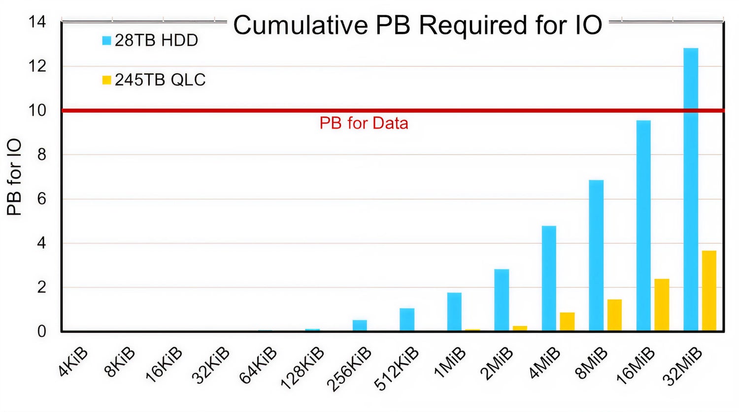 Figure 1. Read and write IO size histograms for an example workload.
(click image to enlarge)
Workload IO histogram: Why it matters
Figure 1 illustrates the distribution of read and write IO sizes for our sample workload. As an object store for HDDs, it primarily writes data in 4 MiB chunks to achieve high throughput. Reads, however, follow a log-normal distribution, peaking at 1MiB but often smaller due to ranged read operations (the large write chunk size often results in the packing of small objects). These smaller reads and writes can significantly affect storage device performance, particularly for HDDs, which are less efficient at handling small IO sizes.
Because HDD performance degrades sharply at small IO sizes, write caching is commonly used to reduce the number of small writes reaching the disk. Write caching is often used to mitigate the impact of small write operations. For our example, let's assume the cache absorbs all write I/O operations of 128 KiB or smaller. This means that only larger writes reach the disk itself. On the read side, not all small read operations will hit data in the cache; let's estimate a 75% cache hit ratio.
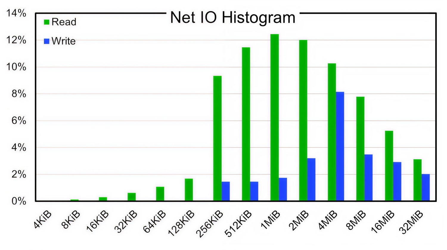 Figure 2. Disk IO histogram after write caching.
(click image to enlarge)
Applying the write cache alters the workload seen by the disk, as shown in Figure 2. A substantial fraction of the small IO has been eliminated from the HDD. Even the small amount of remaining small reads can be a performance bottleneck for HDDs.
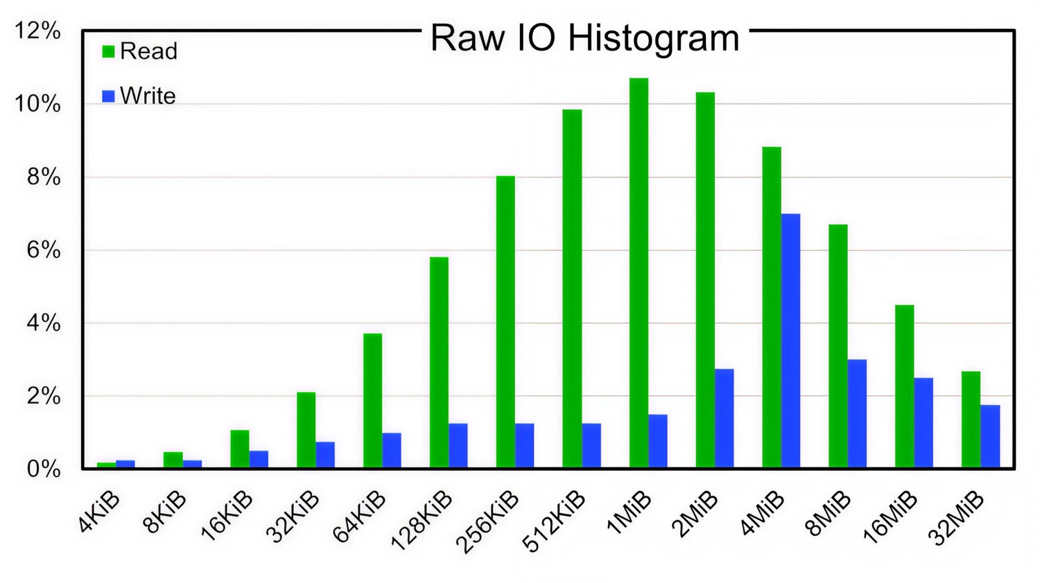 Figure 3. The cumulative PB required to deliver the histogram throughput for the combined read and write workloads.
(click image to enlarge)
Capacity required to meet the workload histogram
Given the effective IO histogram seen by each device, the next step is to determine how much physical capacity is required to sustain the workload throughput. The next step is to calculate the physical storage capacity required to meet these demands. For HDDs, we use the net IO histogram (after caching) for this calculation. QLC flash, on the other hand, handles small IO sizes much more efficiently, so we use the raw histogram without adjustment. This distinction is crucial: QLC can deliver higher throughput for small I/O sizes, which can translate into fewer drives and lower overall system cost for workloads dominated by small reads and writes. Table 1 summarizes the number of drives required to meet both data capacity and IO throughput for the same workload.
Figure 3 shows the cumulative PB required to deliver the throughput at each IO size, computed using the IO histogram and the TB for 1MB/s curve. The 10PB workload data requirement is shown as the red line, and the 28TB HDD exceeds it.
QLC performance and cost advantage
You can clearly see that the QLC requires less capacity to deliver the same IO. In this case, our 10,000 TB system requires:
| Drive type | Drives for data | Drives for IO | % Drives for IO | Watts | Watts/data PB |
|---|---|---|---|---|---|
| 28TB HDD | 357 | 458 | 128% | 3,890 | 389 |
| 245 TB QLC | 41 | 15 | 37% | 1,230 | 123 |
Even though the overall throughput density is 6 MB/s/TB here, achieving this with 28 TB HDDs requires 28% more HDDs and still provides only 10,000 TB of usable space.
QLC, however, uses only about 37% of the available performance and 32% of the HDDs' power. So, if the drive $/TB for QLC is 4x higher than HDD, a 1.28x increase in HDD capacity reduces this to 3.1x, without accounting for other effects.
Conclusion
IO size distribution drives the real storage requirement.
In this example, the QLC SSD example uses about one-third the power of the HDD example: 1,230W versus 3,890W. In addition to this power differential, the HDDs also need 28% more physical drives to meet the IO requirement, while QLC meets the same workload with headroom.
That changes the cost and value comparisons.
For object workloads with meaningful small-IO content, raw media $/TB does not capture the deployed system. Cost per usable PB is the better comparison point because it reflects the drives, power and performance needed to serve the workload.
By that measure, QLC can be closer to HDD than the starting $/TB comparison suggests.